Today’s evidence is not new; is, in fact, well known. Well, make that just plain known. It’s learned and then forgotten, dismissed. Everybody knows about these kinds of mistakes, but everybody is sure they never happen to them. They’re too careful; they’re experts; they care.
It’s too easy to generate “significant” answers which are anything but significant. Here’s yet more—how much do you need!—proof. The pictures below show how easy it is to falsely generate “significance” by the simple trick of adding “independent” or “control variables” to logistic regression models, something which everybody does.
Let’s begin!
Recall our series on selling fear and the difference between absolute and relative risk, and how easy it is to scream, “But what about the children!” using classical techniques. (Read that link for a definition of a p-value.) We anchored on EPA’s thinking that an “excess” probability of catching some malady when exposed to something regulatable of around 1 in 10 thousand is frightening. For our fun below, be generous and double it.
Suppose the probability of having the malady is the same for exposed and not exposed people—in other words, knowing people were exposed does not change our judgment that they’ll develop the malady—and answer this question: what should any good statistical method do? State with reasonable certainty there aren’t different chances of infection between being exposed and not exposed groups, that’s what.
Frequentist methods won’t do this because they never state the probability of any hypothesis. They instead answer a question nobody asked, about some the values of (functions of) parameters in experiments nobody ran. In other words, they give p-values. Find one less than the magic number and your hypothesis is believed true—in effect and by would-be regulators.
Logistic regression
Logistic regression is a common method to identify whether exposure is “statistically significant”. Readers interested in the formalities should look at the footnotes in the above-linked series. Idea is simple enough: data showing whether people have the malady or not and whether they were exposed or not is fed into the model. If the parameter associated with exposure has a wee p-value, then exposure is believed to be trouble.
So, given our assumption that the probability of having the malady is identical in both groups, a logistic regression fed data consonant with our assumption shouldn’t show wee p-values. And the model won’t, most of the time. But it can be fooled into doing so, and easily. Here’s how.
Not just exposed/not-exposed data is input to these models, but “controls” are, too; sometimes called “independent” or “control variables.” These are things which might affect the chance of developing the malady. Age, sex, weight or BMI, smoking status, prior medical history, education, and on and on. Indeed models which don’t use controls aren’t considered terribly scientific.
Let’s control for things in our model, using the same data consonant with probabilities (of having the malady) the same in both groups. The model should show the same non-statistically significant p-value for the exposure parameter, right? Well, it won’t. The p-value for exposure will on average become wee-er (yes, wee-er). Add in a second control and the exposure p-value becomes wee-er still. Keep going and eventually you have a “statistically significant” model which “proves” exposure’s evil effects. Nice, right?
Simulations
Take a gander at this:

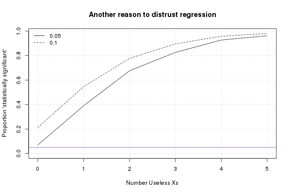
Follow me closely. The solid curve is the proportion of times in a simulation the p-values associated with exposure were less than the magic number as the number of controls increase. Only here, the controls are just made up numbers. I fed 20,000 simulated malady yes-or-no data points consistent with the EPA’s threshold (times 2!) into a logistic regression model, 10,000 for “exposed” and 10,000 for “not-exposed.” For the point labeled “Number of Useless Xs” equal to 0, that’s all I did. Concentrate on that point (lower-left).
About 0.05 of the 1,000 simulations gave wee p-values (dotted line), which is what frequentist theory predicts. Okay so far. Now add 1 useless control (or “X”), i.e. 20,000 made-up numbers1 which were picked out of thin air. Notice that now about 20% of the simulations gave “statistical significance.” Not so good: it should still be 5%.
Add some more useless numbers and look what happens: it becomes almost a certainty that the p-value associated with exposure will fall less than the magic number. In other words, adding in “controls” guarantees you’ll be making a mistake and saying exposure is dangerous when it isn’t.2 How about that? Readers needing grant justifications should be taking notes.
The dashed line is for p-values less than the not-so-magic number of 0.1, which is sometimes used in desperation when a p-value of 0.05 isn’t found.
The number of “controls” here is small compared with many studies, like the Jerrett papers referenced in the links above; Jerrett had over forty. Anyway, these numbers certainly aren’t out of line for most research.
A sample of 20,000 is a lot, too (but Jerrett had over 70,000), so here’s the same plot with 1,000 per group:

Same idea, except here notice the curve starts well below 0.05; indeed, at 0. Pay attention! Remember: there no “controls” at this point. This happens because it’s impossible to get a wee p-value for sample sizes this small when the probability of catching the malady is low. Get it? You cannot show “significance” unless you add in controls. Even just 10 are enough to give a 50-50 chance of falsely claiming success (if it’s a success to say exposure is bad for you).
Key lesson: even with nothing going on, it’s still possible to say something is, as long as you’re willing to put in the effort.3
Update You might suspect this “trick” has been played when in reading a paper you never discover the “raw” numbers, where all that is presented is a model. This does happen.
———————————————————————
1To make the Xs in R: rnorm(1)*rnorm(20000); the first rnorm is for a varying “coefficient”. The logistic regression simulations were done 1,000 times for each fixed sample size at each number of fake Xs, using the base rate of 2e-4 for both groups and adding the Xs in linerally. Don’t trust me: do it yourself.
2The wrinkle is that some researchers won’t keep some controls in the model unless they are also “statistically significant.” But some which are not are also kept. The effect is difficult to generalize, but in the direction of we’ve done here. Why? Because, of course, in these 1000 simulations many of the fake Xs were statistically significant. Then look at this (if you need more convincing): a picture as above but only keeping, in each iteration, those Xs which were “significant.” Same story, except it’s even easier to reach “significance”.
3The only thing wrong with the pictures above is that half the time the “significance” in these simulations indicates a negative effect of exposure. Therefore, if researchers are dead set on keeping on positive effects, then numbers (everywhere but at 0 Xs) should be divided by about 2. Even then, p-values perform dismally. See Jerrett’s paper, where he has exposure to increasing ozone as beneficial for lung diseases. Although this was the largest effect he discovered, he glossed over it by calling it “small.” P-values blind.
Discover more from William M. Briggs
Subscribe to get the latest posts sent to your email.
Sorry, but as a criticism of “P-values” this is just wrong. I don’t know whether the error is in your simulation or in something published by the EPA, but in a large simulation with no built in “effect”, the frequency of an apparent “effect” *is* (on average) the P-value. Any consistent difference from that just means that someone made a mistake in calculating the P-value for the simulation.
Alan,
Actually, this is just classic example of (ludicrous) over-fitting, brought on by the very low probability of “exposure” in combination with a very large sample size. The model (and therefore simulation) is wrong, as you suggest: it should never have been run. But that it shouldn’t doesn’t, of course, stop people from doing so. Loose analogy is a t-stat, which for a fixed numerator is proportional to (a function of) the sample size. Eventually, as SS increases, wee p-values are reached.
My cosmologist friend told me once that “with seven factors you can fit any set of data. As long as you can play with the coefficients.”
Then, too, I recollect exactly the point of this post made in a Scientific American article from decades ago which pointed out that a multiple correlation in n variables could be improved by adding an n+1 variable, even if it has no relationship whatever to the model. The example used was to add National League batting averages to some physics model; though the details are hazy.
@YOS
“With four parameters I can fit an elephant, and with five I can make him wiggle his trunk. (John von Neumann)
My chances of getting 510 Heads in 1000 tosses of a fair coin is less than of getting 51 Heads in 100 tosses. So it is not surprising that increasing sample size gives wee p-values. But increasing the number of variables measured (eg recording also the last digit on my clock at the time of each throw) should not increase or decrease the p-value. It may change the correlation coefficient in some kind of regression analysis, but if it does so then the cutoff for a “significant” level of correlation must be dependent on the number of variables measured. There’s nothing wrong with that, but if it *is* true then any use of that correlation coefficient must be applied with the appropriate variable-number dependent cutoffs. This really isn’t that hard to do properly!
I agree that this is an example of overfitting. The simulations assumed that the incidence of the outcome is 1 in 5000. The first graph has a total n of 20,000, so there were about 2 events in each exposure group. The usual rule-of-thumb is that to avoid overfitting, you need 10-15 events per independent variable added to the model. With only four events (total for both exposure groups), any multivariable regression will be overfitting and thus generate meaningless and misleading results.
Despite the title of the blog post, these simulations don’t critique P values in general. But they vividly point out that P values from logistic regression are meaningless (and misleading) with very rare events.
Harvey,
Exactly so. Yet it is no surprise that many (many) many people blindly “submit” data to software and believe whatever it tells them. P-value small? Effect must be true. And thus is born another peer-reviewed paper.
Funny thing is that logistic regression doesn’t “break”; i.e. it still gives plausible answers. For instance, in these simulations the “excess” probability of “exposure” was on average as designed.
The problem of overfitting is not that it creates low P-values but that it takes one beyond the range of validity of the “rule” one has assumed for connecting size of correlation coefficients with P-value. If a software package reports a P-value for something that is consistently less than the actual observed frequency of that thing then the software is just wrong (or has been applied in a situation where its documentation should have said it was inapplicable). I am agreeing mostly with Harvey here, but I think it is important to note that what is being represented as “P values from logistic regression” are not actually P-values but just estimates of them via some process which does not work correctly (eg when the number of events per variable is too small).
I also agree with Briggs complaint that “many people blindly “submit†data to software and believe whatever it tells them”. But please let’s identify the problem correctly.
Bonferroni?
Steve, Yes, perhaps that’s on the right track – with the (apparently wrong) implementation of “logistic regression” using something less conservative but inapplicable in the case of completely uncorrelated variables.
P.S. In my previous comment I should have referred to “the actual observed frequency of that thing” as being in the context not of the experiment itself but of a properly run simulation of a situation in which the variables being compared are truly independent (ie in a context where the null hypothesis applies).
Pingback: Armed EPA Ignores Subpoena, Conducts Secret Science, More! | William M. Briggs
How would someone prevent making this mistake with Logistic Regression modeling? Is there a power formula that would say I need N=1,000,000 rather than 10,000 per group to detect a significant change from the expected risk of 2/10,000 people harmed with x independent variables?